How To Know The Change Of Temperature On The Meteogram

Meteograms: Messages in Time

Prioritize...

The emphasis of this lesson has been making sense out of all the information available to meteorologists. So far, we have mainly been looking at how to display data that varies in space but has been collected at a unmarried fourth dimension. In this department we will discuss the apply of the meteogram -- a way of displaying a time-history of data from a unmarried station. Upon finishing this section, you should be able to interpret meteograms from both Unisys and the University of Wyoming.

Read...

For most of this lesson nosotros accept been looking at how to ameliorate visualize data in infinite (at a single fourth dimension). In this section, we're going to change gears and wait at how to visualize a serial of observations (over a catamenia of time) at a single station. For the record, a meteogram (formally called a meteorogram) typically displays observed or predicted atmospheric variables (temperature, dew betoken, current of air, etc.) at a unmarried station over a period of time (usually 24 hours or, 25 hourly weather observations). While there is no "official" ready of rules for creating a meteogram, many of the ones that you volition discover on the Internet share some mutual characteristics. The important concept here is to know what a meteogram is showing (in general) and so sort out where/how all of the diverse pieces of data are displayed. We will look at the ii nearly common meteograms: those produced by the University of Wyoming and, those establish on the Unisys website.

University of Wyoming Meteograms

Meteograms from the University of Wyoming Atmospheric Sciences website tin be generated for a broad variety of times and locations. To create your own meteograms from this Spider web site, first use the menu on the left to choose a region of interest. In the second bill of fare (from the left) scroll downwardly and select "GIF Meteogram". Then click on the dot representing the city or town of interest on the map displayed. What will appear is a meteogram like the sample below.

A University of Wyoming meteogram from Pittsburgh International Airport.

A sample meteogram from the Web site at the Academy of Wyoming for Pittsburgh International Airport on May 19-20, 2003. Courtesy of University of Wyoming.

To first affair to do before diving into the data is to get your bearings. Find that the times and dates covered by the meteogram appear at the bottom of the image. This meteogram from Pittsburgh, Pennsylvania, spans from 1951Z on May 19, 2003 to 1851Z on May 20, 2003. Notation the "tic" marks (short, vertical line segments) forth the lesser of the first rectangular plot. Each "tic" mark represents a "synoptic time". By convention, "synoptic times" are 00Z, 03Z, 06Z, 09Z, 12Z, 15Z, 18Z, and 21Z. So, on this detail meteogram from Pittsburgh, the first "tic mark" represents 21Z on May 19, the starting time synoptic time afterward 1951Z on May nineteen. The second from the left "tic mark" corresponds to 00Z on May 20; the third from the left corresponds to 03Z; and and so on and and so forth. Merely in case y'all take trouble, note that the dates and times are explicitly listed beneath the "tic marks" along the base of operations of the 3rd rectangular plot at the lesser of the meteogram.

Next turn your attention to the three traces on the upper rectangular graph. The purplish plot represents the variation of surface air temperatures with time. The greenish plot shows the time variation of surface dew points. The bluish plot marks the variation of surface relative humidity with time. Beneath the first rectangular graph, the serial of purplish numbers represents the hourly surface air temperatures. Below the hourly temperatures, the green symbols represent precipitation and other restrictions to visibility. These symbols are the aforementioned ones that announced on conventional station models (notation the moderate rain observed at the Pittsburgh airdrome at 15Z on May 20.)

Below weather and restrictions to visibility, the brownish station models allow yous to assess deject cover, surface current of air management and surface wind speed in the same manner as you would with a typical station model. When winds are gusty, the maximum wind gust is reported straight higher up the station model. For case, at 01Z on May 20, the maximum wind gust at Pittsburgh International Airdrome was sixteen knots.

The second rectangular graph includes a plot of horizontal visibility with time (the brown plot). In this case, the visibility at Pittsburgh was 10 miles (read off the scale on the right) from 1951Z on May xix to 15Z on May 20. Once it started to rain, visibility decreased rapidly, bottoming out at ii miles between 16 and 17Z on May xx. The scale on the left represents the heights of cloud bases in feet. Earlier we talk nigh how clouds are represented on a meteogram, permit me have a quick detour to introduce you to cloud nomenclature.

There are four general classifications of clouds: high, middle, and depression clouds likewise as clouds of vertical development. The table below summarizes each of these classifications while giving you a sense for the typical altitudes at which their cloud ceilings (the height of their bases) are observed. We'll discuss cloud classification in more detail (including their individual names) later in the course.

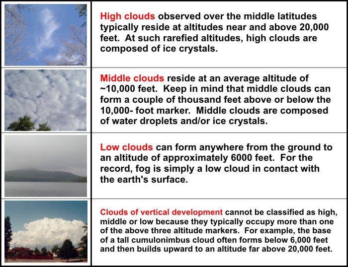
The 4 general classifications of clouds. Photos Credit: David Babb

Now back to the meteogram. Note that there are several letters located at each time flow. These letters correspond deject layers. The pinnacle of the layer is represented by where the letter is placed (call up the elevation scale is to the left). The amount of cloud coverage by each layer is represented by the letter of the alphabet itself ("O" -- clouded; "S" -- scattered; "B" -- broken). There is too the modifier, "-" , which can be interpreted "lightly". So, at 19Z on May 19, it was overcast over Pittsburgh (note the "O") above 10,000 feet, suggesting an overcast of mid-level or high clouds. An hour later on at 20Z, clouds were "lightly scattered" (that is, "few") at 10,000 anxiety, suggesting some mid-level clouds, and above ten,000 feet, clouds were cleaved. Finally, at 16Z on May 20 (rain had started at Pittsburgh), clouds clouded at 3,000 feet (depression clouds) with a scattered layer between 1000 and 3000 anxiety.

Beneath the 2nd rectangular plot at 00Z, 06Z and 12Z, you'll detect the highest temperature during the previous six-hr period (in the purplish colour). The greenish temperatures at these synoptic times represent the lowest temperature during the previous vi-60 minutes period. The next entry corresponds to the amount of liquid atmospheric precipitation observed in the six-60 minutes catamenia ending at 00Z, 06Z, 12Z, or 18Z. In this case, 0.21 inches of pelting fell at Pittsburgh in the half dozen-60 minutes period catastrophe at 18Z on May 20. And finally, the third rectangular plot shows the time variation in barometric pressure.

Meteograms from Unisys

The meteogram below from the interactive website at Unisys shows the evolution of a series of atmospheric condition observations taken at the Philadelphia International Airport from 13Z on August 18, 2011, to 13Z on August 19, 2011. The layout of Unisys meteograms is slightly different than the format of Wyoming'southward meteograms. They are not quite equally comprehensive as the University of Wyoming, but they certainly have a dainty look. The header includes only the station identifier. For this example, KPHL translates to the Philadelphia International Airport.

A Unisys meteogram from Pittsburgh International Airport.

A standard meteogram from the Web site at Unisys documents conditions observations at the Philadelphia International Airport from 13Z on August 18, 2011, to 13Z on August 19, 2011. Courtesy of Unisys.

The topmost graph on Philadelphia's meteogram contains traces of temperature (upper, green trace) and dew point (lower, blue trace) during the previous 24-60 minutes menstruation (25 hourly observations). Annotation the times along the lesser which are explicitly labeled. I also point out that, different meteograms from the University of Wyoming, Unisys meteograms don't include relative humidity in the topmost graph.

A close-up of a Unisys meteogram highlighting the lines of weather data beneath the temperature graph.

An annotated close-up of the lines of weather data below the plots of temperatures and dew points on meteograms from the Unisys Web site.

Below the topmost plots of temperatures and dew points, several kinds of weather data are displayed. The annotated generic close-up on the left decodes these lines of various weather data. The label, "EXTT", designates extreme temperatures (highest and everyman readings during a standard catamenia of time). Note that most of the temperatures appear at the main synoptic times (00Z, 06Z, 12Z, 18Z), with readings at 18Z and 00Z representing the highest temperature observed during the vi-hour menstruum ending at 18Z and 00Z. The farthermost temperatures reported at 06Z and 12Z represent the lowest readings observed during the six-hour period ending at 06Z and 12Z. The 87 degrees reported at 05Z (not a synoptic fourth dimension) was the high temperature recorded on August xviii, 2011.

Next, the atmospheric condition category, "WX", indicates present weather (precipitation or obstructions to visibility, such as fog and haze). Annotation the thunderstorm symbols at KPHL around 00Z and 06Z. To the far correct of "PREC," the 24-60 minutes rainfall catastrophe at 12Z on the 19th was 1.52 inches. The other reported rainfalls stand for half dozen-hour totals catastrophe at the main synoptic times. For case, the "0.73" reported at 06Z on the 19th indicates that 0.73 inches of rain brutal during the 6-hour period ending at 06Z.

A fourth dimension-sequence of horizontal visibility follows precipitation (measured in statute miles), and below that, a fourth dimension-evolution of wind gusts, measured in knots, documents the wind's unsteadiness. Fourth dimension slots are left empty if the wind is relatively steady. Familiar station-model conventions for representing wind direction and speed appear below the air current gusts. Note the familiar shading of role or all of the station circumvolve, indicating the coverage of clouds. The same convention for sky comprehend that you learned for standard station models besides applies here.

Unisys meteograms display clouds and cloud ceilings a bit differently than the University of Wyoming. The altitude, in anxiety, of the base of operations of an observed deject layer tin be gleaned from the vertical list of numbers on the left (delight keep in mind that that these heights are not linearly spaced). Horizontal dashes are used to designate deject layers. If the observed cloud layer is scattered when the weather observer assesses the land of the sky, then it's represented past a single, brusk dash at the altitude of its base. Ii curt dashes at the advisable altitude are used if the cloud layer is broken, while a single, long nuance designates an overcast layer. When the sky is clear, "C" appears on the meteogram at the hr of observation, while, when the heaven is obscured, "X" is plotted on the meteogram. Call back that, when the sky is obscured, heavy rain, heavy snow, thick fog, thick smoke, thick haze, etc. prevents the observer from determining the state of the sky.

Finally, the last graph in the meteogram is a time trace of mean ocean-level force per unit area (in mb).

Case Study...

The meteogram below, which comes courtesy of the University of Wyoming, shows conditions conditions at Phoenix, Arizona (Heaven Harbor International Airdrome) from 22Z on July v, 2011, to 23Z on July half dozen, 2011.

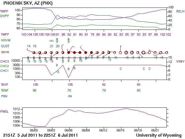
A University of Wyoming meteogram from Phoenix, Arizona.

A meteogram from the Web site of the University of Wyoming shows weather atmospheric condition at Phoenix's Heaven Harbor International Airport from 22Z on July 5, 2011, to 23Z on July 6, 2011. Courtesy of the University of Wyoming.

What stands out on this meteogram? Well, information technology was a "routinely" hot July afternoon and early evening at Phoenix. Indeed, temperatures (designated by the purple plot on the topmost graph and labeled TMPF for "temperature in degrees Fahrenheit"), sizzled in a higher place 100 degrees from 22Z on the 5th to 03Z on the 6th. Then, from 03Z to 04Z (8 P.Grand. to ix P.G. MST), the mercury abruptly plummeted to 81 degrees with gusty winds (the fifth characterization from the top, GUST, displays wind gusts in knots). To the correct of WSYM, which designates electric current weather and restrictions to visibility, notice what looks like a dollar sign at 04Z . If you peruse the list of symbols for present atmospheric condition, you'll come across that this "dollar sign" represents a sandstorm. And what a sandstorm it was...bank check out this YouTube video of the weather in Phoenix at this time.

I similar to collect compelling meteograms like the i at Phoenix, and the summertime of 2011 provided enough of good examples. Check out the meteogram (below) from Westfield Barnes Airport (KBAF) near Westfield, Massachusetts, from 21Z on May 31, 2011, to June i, 2011. In example you're wondering, the symbol to the extreme correct of weather and restrictions to visibility (WSVM) represents a funnel cloud / tornado (check out the YouTube video of the Westfield tornado).

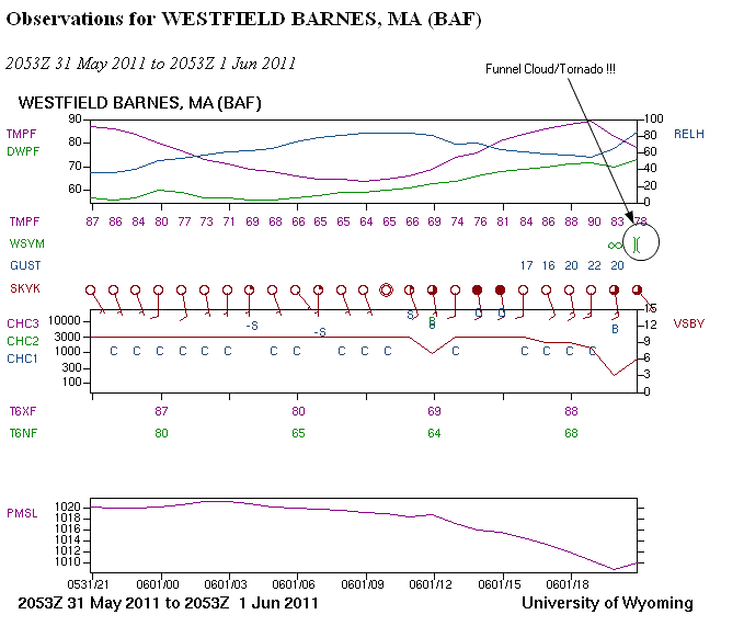
A University of Wyoming meteogram from Westfield Barnes, MA.

The meteogram at the Westfield Barnes Airport (KBAF) near Westfield, Massachusetts, from 21Z on May 31, 2011, to 21Z on June ane, 2011. Note the symbol for a funnel deject / tornado at 21Z on June 1. Courtesy of Academy of Wyoming.